
The short version: the regression itself is four clicks. Everything that decides whether your results chapter survives happens in the boxes you tick before you click OK, and in what you do when an assumption fails. This guide covers the whole run — dialog, diagnostics, rescues, table, sentence.
One note on sourcing before we start. IBM’s own SPSS documentation was unreachable from here in August 2026, returning a 403 to one instrument and a 503 to another, so the dialog descriptions below are written to be checked against the software in front of you rather than quoted from the vendor. Labels shift slightly between versions; the structure has not changed in years.
Step 1: Get the variables right before you open anything
- Confirm the outcome is continuous. If it is binary, you need logistic regression, and running linear regression on a 0/1 outcome is the single most common misuse an examiner catches immediately.
- Dummy-code every categorical predictor. A four-category variable becomes three 0/1 indicators, and the omitted category is your reference. Write down which category you omitted, because every coefficient is now interpreted against it, and you will need that sentence in your write-up.
- Decide the missing-data rule now, not later. SPSS defaults to listwise deletion, which quietly drops any case with a gap on any variable in the model. Check the N in your output against the N in your sample. If they differ, that difference is a methods-chapter sentence, not a rounding error.
- Sanity-check your N against your number of predictors. Common rules of thumb suggest at least 10 to 20 cases per predictor. They are conventions, not standards, and a real power analysis for your expected effect size is the defensible version.

Step 2: Run it, and tick the boxes you will otherwise have to come back for
The dialog is Analyze → Regression → Linear. Put the outcome in Dependent and your predictors in Independent(s). Leave the method on Enter unless you have a stated reason to do otherwise — stepwise methods let the software choose your model, which is a decision an examiner will ask you to justify and which you generally cannot.
Then, before OK, open the sub-dialogs:
- Statistics: Estimates · Confidence intervals · Model fit · Collinearity diagnostics · Durbin-Watson · Casewise diagnostics.
- Plots: put
*ZRESIDon the Y axis and*ZPREDon the X axis, and tick the Normal probability plot. That single scatterplot tests two assumptions at once. - Save: Cook’s distance, and standardised residuals. These are written back as new columns so you can find the offending cases by row rather than by squinting.
Ticking all of these on the first run costs ten seconds and saves you re-running the model at 1 a.m. three weeks later when your supervisor asks about multicollinearity.
Step 3: Check the five assumptions
| Assumption | Where you look | Conventional signal |
|---|---|---|
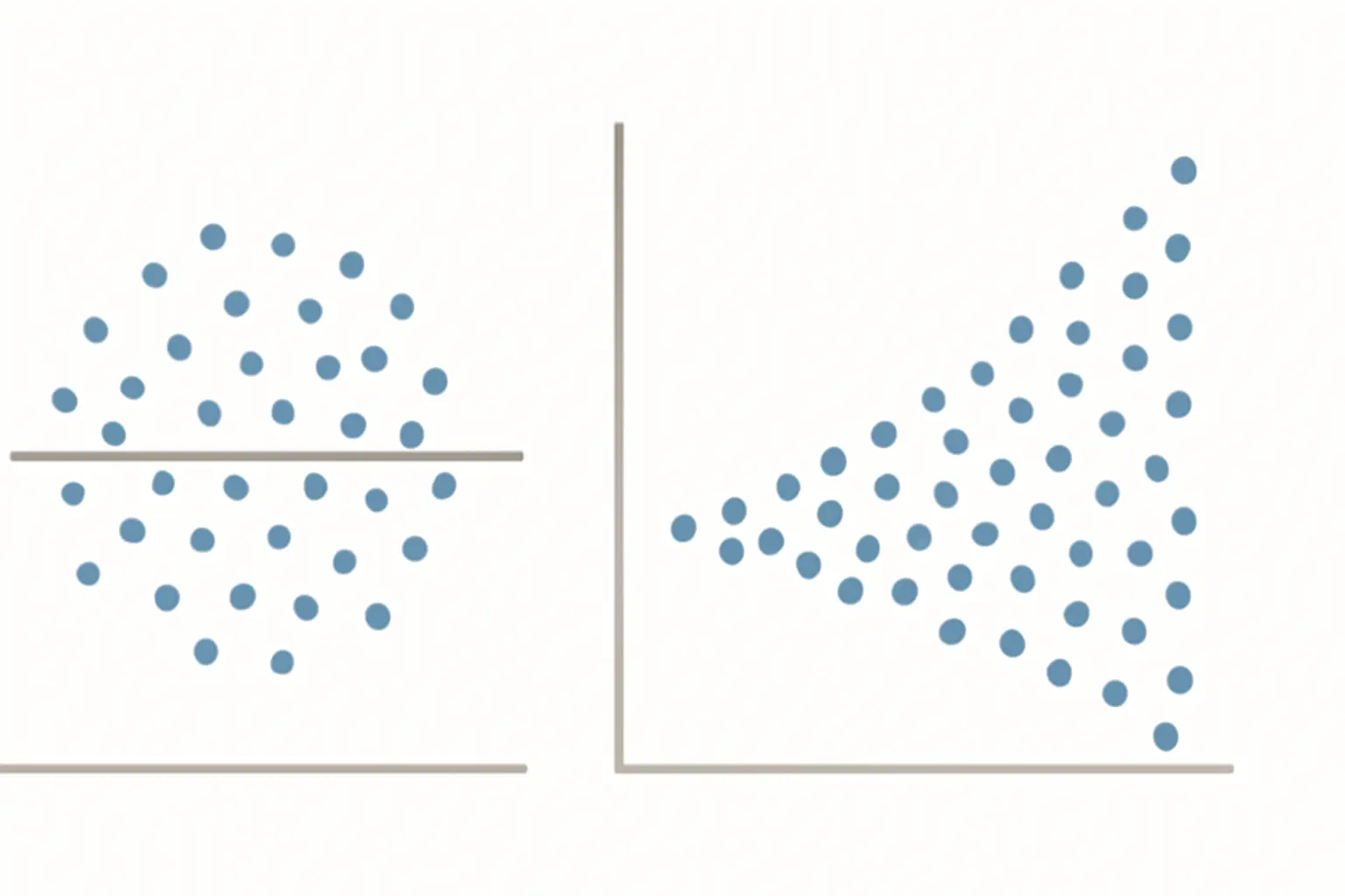
| Linearity | The *ZRESID × *ZPRED scatterplot |
A shapeless cloud. A curve means the relationship is not linear |
| Homoscedasticity | The same scatterplot | Even vertical spread. A widening wedge is heteroscedasticity |
| Independence of residuals | Durbin-Watson, in Model Summary | Roughly 1.5 to 2.5 is usually treated as unremarkable |
| No serious multicollinearity | VIF and Tolerance, in Coefficients | VIF above 10 (some fields use 5) or Tolerance below .10 |
| Normally distributed residuals | Normal P-P plot of residuals | Points close to the diagonal. Note: residuals, not your variables |
Two clarifications that save real confusion. Regression does not assume your predictors or your outcome are normally distributed — it assumes the residuals are, which is why the P-P plot is of residuals and why running a Shapiro-Wilk on your raw variables answers a question nobody asked. And every threshold in that table is a convention, not a standard: VIF of 10 and VIF of 5 are both defended in print, so state which you used and why.
Separately, check Cook’s distance for influential cases. A value above 1 is the usual flag. An influential case is not automatically an error to be deleted; it is a case to be looked at, and if you remove it you report the model with and without it.
Step 4: What to do when an assumption fails
This is the section students actually need at 11 p.m., and the one most tutorials skip. A failed assumption is not a failed analysis. Each failure has a standard response, and using it — and saying you used it — is stronger than pretending the plot looked fine.
| What failed | What it does to your results | The standard response |
|---|---|---|
| Heteroscedasticity | Coefficients stay unbiased; standard errors and therefore p values are wrong | Bootstrap the model (SPSS Bootstrap sub-dialog, 1,000–5,000 resamples) and report the bootstrapped confidence intervals, or use heteroscedasticity-consistent standard errors |
| Non-normal residuals | Matters mainly in small samples; inference is affected more than estimates | Bootstrap the confidence intervals. With a large N the central limit theorem does most of this work already — say so rather than transforming for no reason |
| Non-linearity | The model is answering the wrong functional question | Transform the predictor, add a quadratic term, or move to a model that fits the shape. Do not report a linear slope through a curve |
| Multicollinearity (VIF high) | Individual coefficients become unstable; the overall model can still fit well | Combine the collinear predictors into one index, drop one on theoretical grounds, or centre the variables if the collinearity comes from an interaction term |
| Autocorrelated residuals | Standard errors are wrong; usually a sign of clustered or time-ordered data | Model the structure — a time-series model, or a multilevel model if cases are nested in schools, clinics or classes |
| Influential cases | One respondent may be driving a coefficient | Report the model with and without the case, and let the reader see that the conclusion does not depend on one person |
Notice the pattern: bootstrapping fixes two of the six, and it is three clicks in SPSS. If you learn one rescue, learn that one.
Step 5: Read the three tables
Model Summary gives R and R². R² is the proportion of variance in the outcome accounted for by the model. Report adjusted R² alongside it, because plain R² rises every time you add a predictor whether or not the predictor is doing anything.
ANOVA gives the omnibus F test: is the model as a whole better than predicting the mean for everybody? A non-significant F with a significant individual coefficient is a warning sign, not a result.
Coefficients is the table you will report. Per predictor: B (the unstandardised coefficient — the change in the outcome for a one-unit change in the predictor, holding the others constant), its standard error, β (the standardised coefficient, comparable across predictors on different scales), t, the p value, the confidence interval, and your collinearity statistics.
Which coefficient to lead with depends on your question. If your predictor has a meaningful unit — years, dollars, milligrams — B is more informative and should be interpreted in that unit. If you are comparing the relative contribution of predictors measured on arbitrary scales, β is the one.
Step 6: Build the APA table
An APA-style table uses horizontal rules only — no vertical lines, no interior grid — with a numbered title in italics above it and any notes below.

| Predictor | B | SE | β | t | p | 95% CI |
|---|---|---|---|---|---|---|
| (Constant) | 2.14 | 0.38 | — | 5.63 | < .001 | [1.39, 2.89] |
| Workload hours | −0.21 | 0.05 | −.34 | −4.20 | < .001 | [−0.31, −0.11] |
| Perceived support | 0.44 | 0.09 | .31 | 4.89 | < .001 | [0.26, 0.62] |
| Years in post | 0.03 | 0.04 | .05 | 0.75 | .454 | [−0.05, 0.11] |
Four formatting rules that a marker will notice. Statistical symbols that are not Greek letters are italicised — M, SD, t, p, B, F, R. Test statistics and p values are conventionally rounded to two decimal places, though exact p values are often given to two or three. A p value below .001 is written as p < .001 rather than as an exact figure. And state your alpha level once, early — “an alpha level of .05 was used for all tests” — rather than implying it.
The reference-list side of formatting, including the four Canadian source types APA does not cover, is a separate job handled in our complete APA 7 guide for a Canadian thesis.
Step 7: Write the sentence
Report the model, then the predictors, then the meaning. A template you can adapt directly:
A multiple linear regression was conducted to predict burnout from workload hours, perceived support and years in post. The model was significant, F(3, 210) = 24.61, p < .001, and accounted for 26% of the variance in burnout (R² = .26, adjusted R² = .25). Workload hours (β = −.34, p < .001) and perceived support (β = .31, p < .001) were significant predictors; years in post was not (β = .05, p = .454). Each additional weekly hour of workload was associated with a 0.21-point decrease in burnout score, holding the other predictors constant.
Then one sentence on diagnostics, which is where most students under-report and lose easy credit:
Assumptions were checked before interpretation. Residuals were approximately normally distributed and independent (Durbin-Watson = 1.94), and no predictor showed problematic multicollinearity (all VIF < 2.1). Inspection of the residual plot indicated mild heteroscedasticity, so confidence intervals were bootstrapped with 5,000 resamples; the reported intervals are the bootstrapped ones.
That second paragraph does something specific for you: it converts an assumption failure from a hidden weakness into visible methodological competence, and it pre-answers the question. Which matters, because “how did you check your assumptions?” is one of the standard question types set out in our guide to what gets asked at a Canadian thesis defence.
Two things to settle around the analysis
Save the syntax. SPSS’s Paste button converts every dialog choice into commands. A script is what lets you re-run the model with one case excluded in four minutes during corrections rather than reconstructing twelve dialog boxes from memory. Whether SPSS is even the right environment for your project — and what happens to your files when the institutional licence lapses — is covered in our comparison of SPSS, R, jamovi and Stata for a Canadian thesis.
Report the reliability of your scales before the regression. If your predictors are questionnaire scales, their internal consistency belongs in the results chapter ahead of the model, because a coefficient built on an unreliable measure is attenuated by construction — our guide to acceptable Cronbach’s alpha values covers what to report and what to do when yours is low.
Once the numbers exist, they still have to become a chapter an examiner can follow. Draft your results chapter in Tesify and keep tables, references and structure consistent while every interpretation remains 100% written by you.
Frequently asked questions
Where is multiple regression in SPSS?
Analyze → Regression → Linear. Put the continuous outcome in Dependent and your predictors in Independent(s), and leave the method on Enter unless you can justify otherwise.
What VIF value is too high?
A VIF above 10 is the most commonly cited flag, with a tolerance below .10 meaning the same thing. Some disciplines use 5. Both are conventions, so state which you applied.
Does regression assume my variables are normally distributed?
No. It assumes the residuals are approximately normal. Testing the raw variables for normality answers a different question.
My residual plot fans out. Is my analysis ruined?
No. Heteroscedasticity affects standard errors rather than the coefficients themselves. Bootstrap the confidence intervals or use robust standard errors, and report that you did.
Should I report B or beta?
Both in the table. In the text, lead with B when the predictor has a meaningful unit and with beta when you are comparing predictors measured on different scales.
Should I use stepwise regression?
Only with a stated reason. Stepwise methods let the algorithm select your model from your data, which is difficult to defend when an examiner asks why a particular predictor is in it.
What is a good R squared?
There is no threshold. What counts as a large proportion of variance explained differs enormously between fields; report adjusted R squared alongside it and compare against studies in your own literature.
How do I report a non-significant predictor?
The same way as a significant one, with its coefficient and exact p value. Omitting non-significant predictors from the table is selective reporting.
How many participants do I need per predictor?
Rules of thumb of 10 to 20 cases per predictor circulate widely, but they are conventions. A power analysis based on the effect size you expect is what a committee will accept.
What does Durbin-Watson tell me?
Whether the residuals are independent of one another. Values in roughly the 1.5 to 2.5 range are usually treated as unremarkable; values far outside it suggest clustered or time-ordered data that needs a different model.
Can I delete an outlier?
Only with a reason you can state, and you should report the model with and without the case so the reader can see whether the conclusion depends on it.
Do I need to write out the regression equation?
Usually not, unless your programme requires it or the equation itself is the contribution. The coefficient table plus the interpretive sentence carries the information.