
The short version: the ANOVA takes four clicks, and the number SPSS shows you first is often not the one you should report. This guide covers the whole run — dialog, variance check, the choice between the classical F and Welch’s, the matching post hoc, the effect size, and the finished table and sentence.
A sourcing note first. IBM’s own SPSS documentation was unreachable from here in August 2026, returning HTTP 403, so the dialog descriptions below are written to be checked against the software in front of you rather than quoted from the vendor. Menu labels shift a little between versions; the structure has not changed in years.
Step 1: Confirm this is actually a one-way ANOVA
- One categorical independent variable, three or more groups. With exactly two groups you want an independent-samples t test instead — an ANOVA on two groups is not wrong, it is just a t test wearing a different hat.
- One continuous outcome, measured once per participant. If the same people were measured at several time points, you need a repeated-measures design, not this one.
- Independent groups. Each participant appears in exactly one group. Matched pairs, siblings, students nested in classrooms and patients nested in clinics all break this, and clustered data needs a multilevel model.
- Write down the group sizes now. Unequal group sizes are not fatal, but they change which test behaves well, and you will need the numbers for your table anyway.

Step 2: Run it, and tick the boxes you will otherwise come back for
The dialog is Analyze → Compare Means → One-Way ANOVA. Your continuous outcome goes in Dependent List; your grouping variable goes in Factor. Before you click OK, open the sub-dialogs:
- Options: Descriptive · Homogeneity of variance test · Welch · Means plot. Brown-Forsythe is offered alongside Welch; request it if you like, but see Step 4 before you plan to report it.
- Post Hoc: tick Tukey under Equal Variances Assumed and Games-Howell under Equal Variances Not Assumed. Requesting both costs nothing and saves a second run once you know which situation you are in.
- Effect size: recent SPSS releases add an effect-size option to this dialog. If yours does not have one, Step 6 gives you the hand calculation from the table you already have.
Ticking all of these on the first run takes ten seconds. Re-running the analysis three weeks later because your supervisor asked whether variances were equal takes considerably longer.
Step 3: Read the variance situation, not just Levene’s p value
SPSS prints a Test of Homogeneity of Variances, and the student reflex is to treat its p value as a switch: significant means unequal variances, non-significant means equal. That reading is weaker than it looks, and the reason is worth understanding rather than memorising.
Levene’s test is itself a hypothesis test with its own power. With small groups it frequently fails to detect variance differences that are genuinely there, so a non-significant Levene’s is not evidence that your variances are equal — it is often just evidence that you did not have enough data to tell. With very large groups the opposite happens and a trivial difference registers as significant.
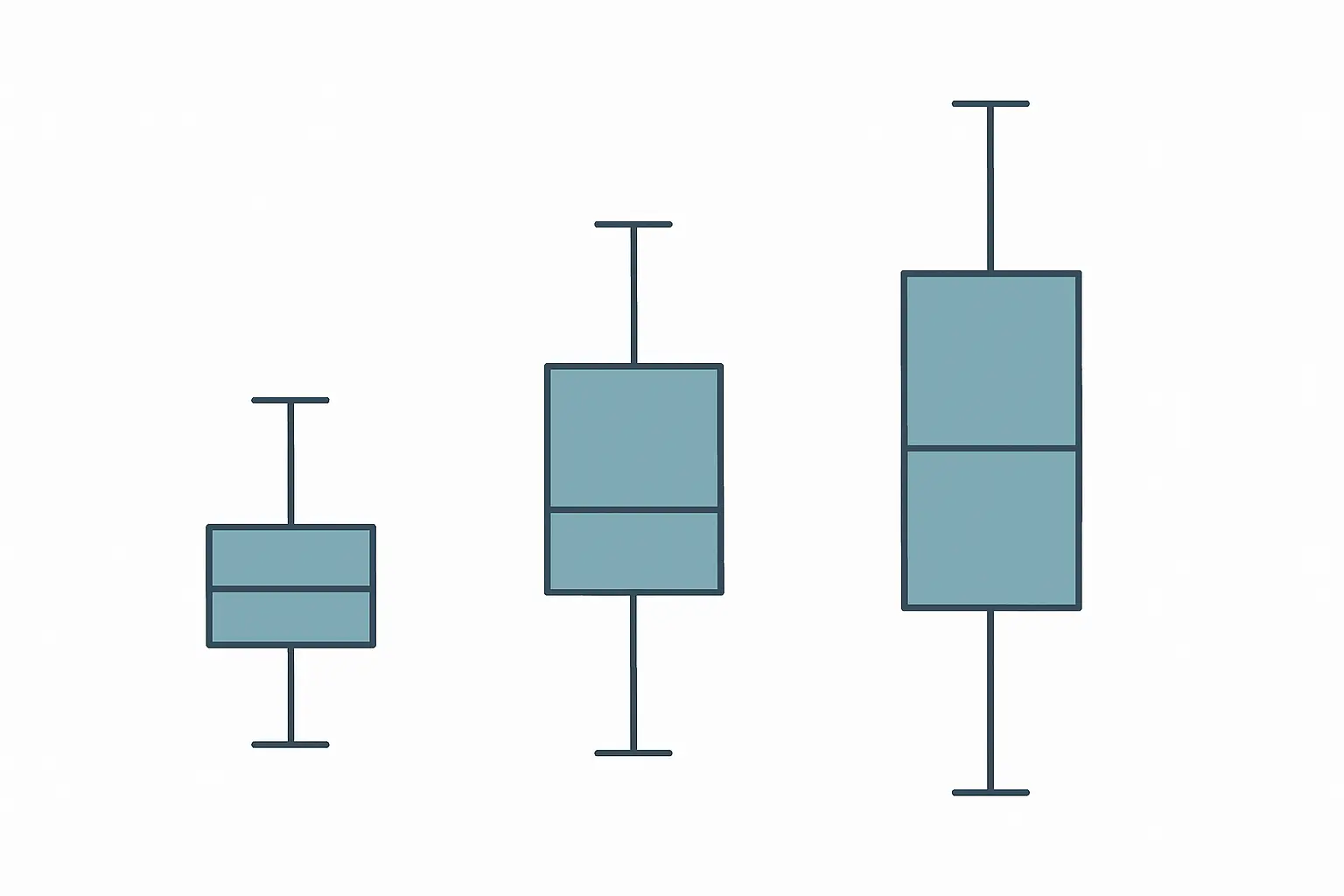
So read three things together: the Levene’s result, the group standard deviations in the Descriptives table, and the boxplots. If one group’s SD is roughly twice another’s, you have a variance problem regardless of what Levene’s says.
Step 4: Decide which omnibus test to report — and consider Welch by default
This is the substantive decision in the whole analysis, and most theses make it by accident, by reporting whatever appeared at the top of the output.
Delacre, Leys, Mora and Lakens set out the case in International Review of Social Psychology (2019, 32(1), article 13, open access). Their Monte Carlo simulations lead to an unambiguous recommendation: use Welch’s W test “by default when comparing means”, and avoid both the classical F test and the Brown-Forsythe F* test. They give four reasons:
- the equal-variances assumption is often unrealistic;
- tests of that assumption “will often fail to detect differences when these are present”;
- the loss of power from using Welch is very small, often negligible;
- the gain in Type I error control is considerable across a wide range of realistic conditions.
The same paper measured how often anyone checks. Of 116 articles in the Journal of Personality and Social Psychology published in 2016, fourteen per cent reported a one-way F test — and exactly one of them indicated that the homogeneity-of-variances assumption had been taken into account. If you report Welch and say why, you are ahead of most of the published literature in your field, which is a good position to be in at a defence.
Two caveats, both from the same authors. They recommend balanced designs — equal group sizes — wherever possible, because Type I error control is generally better. And Welch has a small-sample limit: with fewer than 50 observations per group when comparing at most four groups, or fewer than 100 when comparing more than four, the W test will not control the Type I error rate if the data are skewed. In that situation, check your distributions carefully and consider a trimmed-means or non-parametric alternative.
Step 5: Match the post hoc to the variance situation
The omnibus test tells you only that at least one group differs from at least one other. It does not tell you which, and “the ANOVA was significant so Group 3 is highest” is not a finding.
| Variance situation | Omnibus test to report | Post hoc |
|---|---|---|
| Comparable SDs, balanced groups | Classical F (or Welch, stated) | Tukey HSD |
| Unequal SDs, or unbalanced groups | Welch’s W | Games-Howell |
| Skewed data, small groups | Kruskal-Wallis H | Dunn’s test with an adjustment |
| A small set of planned comparisons | Either, stated in advance | Planned contrasts, not a post hoc sweep |
Mixing rows is the error examiners notice: reporting Welch’s F because variances were unequal and then reading Tukey comparisons, which assume they are equal, is internally inconsistent. If you report Welch, report Games-Howell.
That last row matters more than students expect. If your hypotheses named specific group comparisons before you collected data, planned contrasts test exactly those and cost you less power than an all-pairs sweep. The hypotheses you wrote in chapter two are the record of what was planned.
Step 6: Report an effect size
A p value tells the reader whether a difference is detectable, not whether it matters. Two options, both computable from the output you already have:
- Eta squared (η²) = between-groups sum of squares ÷ total sum of squares, both read straight off the ANOVA table. Interpreted as the proportion of variance in the outcome associated with group membership. It is biased upward in small samples.
- Omega squared (ω²) is the less biased alternative and is preferred in several fields. If your output does not print it, say which one you used and why.
If you are converting between an effect size in the literature and the f that a power analysis wants, the relationship is η² = f²/(1 + f²). Whether your achieved sample could detect the effect you found at all is a separate and very answerable question — our guide to how many participants you actually need covers the sensitivity analysis that answers it.
Step 7: Build the APA table
An APA-style table uses horizontal rules only — no vertical lines, no interior grid — with a numbered italic title above it and notes below.

For a one-way design, a descriptives table carries more information for the reader than the ANOVA source table does:
| Group | n | M | SD | 95% CI |
|---|---|---|---|---|
| Undergraduate | 52 | 3.41 | 0.62 | [3.24, 3.58] |
| Master’s | 48 | 3.88 | 0.71 | [3.67, 4.09] |
| Doctoral | 44 | 4.26 | 1.19 | [3.90, 4.62] |
Four formatting points a marker will notice. Statistical symbols that are not Greek letters are italicised — M, SD, F, p, n. Test statistics and p values are conventionally given to two or three decimals. A p value below .001 is written p < .001 rather than as an exact figure. And state your alpha once, early. The reference-list side of APA, including the Canadian source types the style guide does not cover, is handled in our complete APA 7 guide for a Canadian thesis.
Step 8: Write the sentence
Report the omnibus test, then the comparisons, then the meaning. A template you can adapt directly, for the unequal-variance case:
Group standard deviations differed substantially (0.62 to 1.19), so Welch’s ANOVA was used rather than the classical F test. The effect of degree level on perceived supervisory support was significant, Welch’s F(2, 84.13) = 11.42, p < .001, η² = .14. Games-Howell comparisons indicated that doctoral students reported higher support than undergraduates (mean difference = 0.85, 95% CI [0.38, 1.32], p < .001); the master’s group did not differ significantly from either.
Two details in that paragraph do most of the work. The fractional denominator degrees of freedom — 84.13 rather than a whole number — are the visible signature of Welch’s correction, and a reader who knows the literature will recognise it immediately. And naming the comparison that was not significant prevents the selective-reporting question before it is asked.
What if the assumptions fail badly?
A failed assumption is not a failed analysis; each failure has a standard response.
| What failed | The standard response |
|---|---|
| Unequal variances | Welch’s W with Games-Howell. Report both, and say why. |
| Strong skew in small groups | Kruskal-Wallis H with Dunn’s post hoc and an adjustment, or a trimmed-means test. |
| Outliers driving a group mean | Report the analysis with and without them, so the reader can see the conclusion does not depend on one case. |
| Cases nested in classes, clinics or sites | Independence is broken. Move to a multilevel model rather than adjusting the ANOVA. |
Save the syntax. SPSS’s Paste button converts every dialog choice into commands. A script is what lets you re-run the whole analysis with one case excluded in four minutes during corrections rather than reconstructing eight dialog boxes from memory. Whether SPSS is the right environment at all — and what happens to your files when an institutional licence lapses — is covered in our comparison of SPSS, R, jamovi and Stata for a Canadian thesis. If your groups come from a national dataset rather than your own recruitment, our guide to Statistics Canada data for a thesis covers the access tier and the weighting caveats that come with it.
Once the numbers exist, they still have to become a chapter a committee can follow. Draft your results chapter in Tesify and keep tables, references and structure consistent while every interpretation remains 100% written by you.
Frequently asked questions
Where is one-way ANOVA in SPSS?
Analyze → Compare Means → One-Way ANOVA. The continuous outcome goes in Dependent List and the grouping variable in Factor.
Should I use Welch or the classical F test?
Delacre and colleagues recommend Welch by default, on the grounds that equal variances are often unrealistic and the power cost of Welch is negligible. State which you used and why, whichever you choose.
What does a significant Levene’s test mean?
That the evidence points to unequal variances. But a non-significant Levene’s does not establish that variances are equal — with small groups it often lacks the power to detect a real difference. Read the group standard deviations too.
Tukey or Games-Howell?
Tukey HSD when the group variances are comparable, Games-Howell when they are not. Pair the post hoc with the omnibus test you reported.
What effect size should I report for an ANOVA?
Eta squared or omega squared. Eta squared is the between-groups sum of squares divided by the total sum of squares, so you can compute it by hand from the table if your version does not print it.
Why are my degrees of freedom not whole numbers?
Because you are reading Welch’s test, which adjusts the denominator degrees of freedom for unequal variances. A fractional df is the signature of the correction.
Can I run ANOVA with unequal group sizes?
Yes, but a balanced design controls Type I error better and is worth aiming for at the recruitment stage.
What do I do if my data are not normally distributed?
With reasonable group sizes, mild non-normality is generally tolerable. With small groups and clear skew, use Kruskal-Wallis with Dunn’s post hoc, or a trimmed-means test, and say so.
Do I need post hoc tests if the ANOVA is not significant?
Usually not, unless you had specific planned contrasts stated before data collection. Running an all-pairs sweep after a non-significant omnibus test is difficult to defend.
How many participants do I need per group?
Whatever an a priori power analysis returns for your expected effect size, alpha and target power. Conventions such as thirty per group are heuristics, not standards.
Can I use ANOVA on Likert items?
On a summed multi-item scale, commonly yes. On a single ordinal item it is contested, and a non-parametric test is easier to defend.
What should I cite for the software?
Cite the SPSS version you actually ran, and cite the methodological source for any non-default choice — Delacre et al. (2019) for the decision to report Welch, for example.