
| Step | What it checks | Tool |
|---|---|---|
| 1. State hypotheses | Directional or non-directional relationship between predictors and outcome | — |
| 2. Check assumptions | Linearity, independence, homoscedasticity, normal residuals, no severe multicollinearity | SPSS, R, or jamovi |
| 3. Run the model | Unstandardized/standardized coefficients, R², F-test | SPSS, R, or jamovi |
| 4. Interpret | Which predictors are significant, effect size, direction | — |
| 5. Write up in APA | Regression equation, table, narrative | — |
A worked example, using fictional and clearly labelled illustrative data, of a standard multiple regression a business administration thesis might run: does training hours and tenure predict a retail employee’s supervisor-rated performance score? The steps below are the same whether your software is SPSS, R, or jamovi — only the menu clicks differ.
Setting up the illustrative study
Illustrative research question (fictional, not a real study): Do training hours completed and years of tenure predict supervisor-rated performance among retail sales associates at a mid-size Canadian retail chain?
Hypothesis: H1: Training hours and tenure significantly predict performance score.
Illustrative sample: n = 60 sales associates, performance score rated 1–100 by supervisors, training hours logged over the prior six months, tenure in completed years. This is a fictional dataset built for illustration; a real thesis would report its own actual sample and response rate.
Choosing how predictors enter the model
Before running the model, decide how the predictors will enter it, and justify that choice in your methodology chapter rather than leaving it to your software’s default. Simultaneous (standard) entry puts all predictors in at once and is the right default when you have no theoretical reason to prioritise one predictor over another, which is the approach used in this worked example. Hierarchical entry adds predictors in theory-driven blocks (control variables first, then variables of interest), which lets you report the additional variance explained by each block — useful when your thesis argument is specifically about whether a variable adds explanatory power beyond known controls. Stepwise entry, where the software selects predictors based on statistical criteria alone, is generally discouraged in thesis-level work because it capitalises on chance patterns in your specific sample and is difficult to justify theoretically to a committee; most methodology textbooks recommend simultaneous or hierarchical entry for a defensible business thesis.
Checking assumptions before you run the model
Multiple regression assumes a linear relationship between each predictor and the outcome, independent observations, homoscedasticity (constant variance of residuals across predicted values), approximately normally distributed residuals, and no severe multicollinearity between predictors. In this illustrative example, a scatterplot of standardized residuals against predicted values shows no obvious funnel shape (homoscedasticity holds), a P-P plot of residuals sits close to the diagonal (residuals approximately normal), and the two predictors correlate at r = .21 with each other — low enough that multicollinearity is not a concern. A commonly used threshold is a Variance Inflation Factor (VIF) below 10 (some methodologists use a stricter cutoff of 5); in this illustrative case both predictors’ VIFs sit at 1.05, well under either threshold.

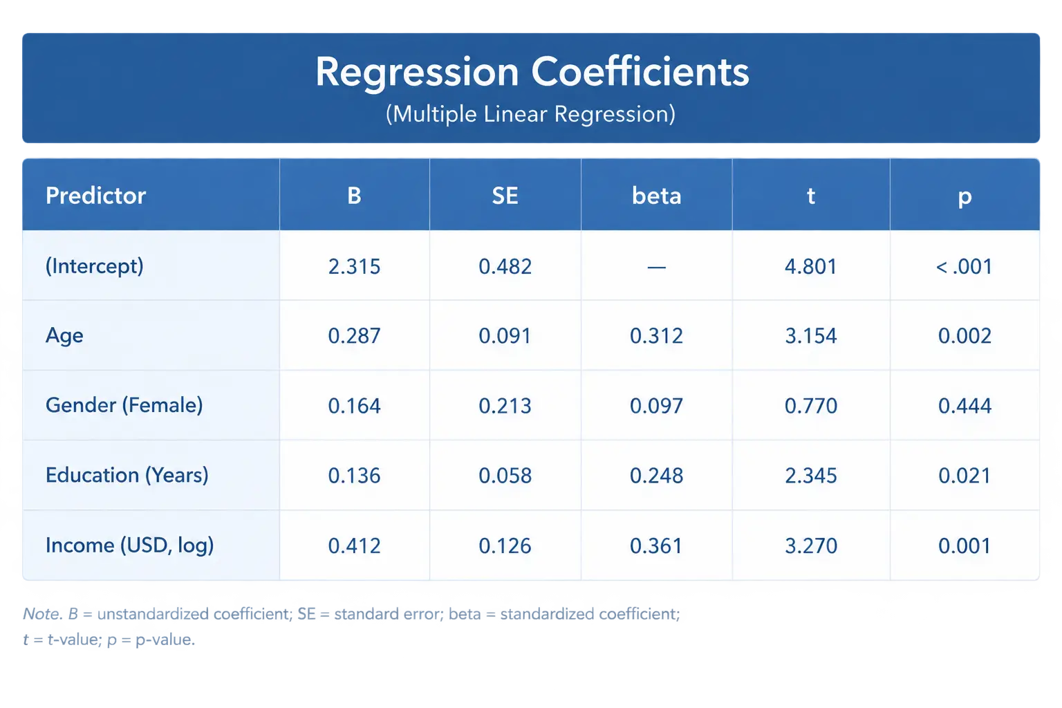
Illustrative regression output
The table below is a fictional, illustrative output built for this worked example, not real study results:
| Predictor | B (unstandardized) | SE | β (standardized) | t | p |
|---|---|---|---|---|---|
| Constant | 52.10 | 4.30 | — | 12.12 | < .001 |
| Training hours | 0.42 | 0.14 | .32 | 3.00 | .004 |
| Tenure (years) | 1.85 | 0.62 | .31 | 2.98 | .004 |
Model summary (illustrative): R = .49, R² = .24, adjusted R² = .21, F(2, 57) = 8.90, p < .001. Note that each t-value above is exactly B divided by its SE (0.42 ÷ 0.14 = 3.00; 1.85 ÷ 0.62 = 2.98, rounded), which is the arithmetic relationship your own output should show as well — if a reported t-value in your real output does not roughly match B/SE, re-check which decimal precision your software is rounding before you assume an error.
Interpreting the illustrative results
In this fictional example, both predictors are statistically significant at p < .01. Training hours has an unstandardized B of 0.42, meaning each additional hour of training is associated with a 0.42-point increase in performance score, holding tenure constant. Tenure has a larger unstandardized B (1.85) because it is measured in years rather than hours, so the standardized coefficients (β = .32 for training hours vs. β = .31 for tenure) are the fairer way to compare their relative contribution — here, almost identical. Together, the two predictors explain 24% of the variance in performance score (R² = .24), a moderate effect in organisational-behaviour research, where R² values in the .10 to .30 range are common given how many unmeasured factors (manager quality, store location, product mix) also affect performance. Using Cohen’s benchmark for the f² effect size in multiple regression (f² = R² ÷ (1 − R²), giving .24 ÷ .76 ≈ .32 here), this illustrative model sits between Cohen’s conventional “medium” (.15) and “large” (.35) thresholds — worth naming explicitly in a discussion section rather than leaving the reader to judge R² = .24 as simply “good” or “weak” without a benchmark.
Writing this up in APA style
Worked example paragraph (illustrative): “A multiple regression was conducted to examine whether training hours and tenure predicted performance score. The overall model was significant, F(2, 57) = 8.90, p < .001, R² = .24, adjusted R² = .21. Training hours significantly predicted performance score, B = 0.42, SE = 0.14, β = .32, t(57) = 3.00, p = .004, as did tenure, B = 1.85, SE = 0.62, β = .31, t(57) = 2.98, p = .004. Together, the predictors accounted for approximately 24% of the variance in supervisor-rated performance.”
Every number in that paragraph traces back to the illustrative table above — the degrees of freedom (57) come from n − k − 1 (60 − 2 − 1 = 57), which is the check to run on your own real output before you write your results paragraph: your reported df should always equal your sample size minus the number of predictors minus one. APA 7th edition style also expects the regression table itself, formatted with the predictor names as row labels and B, SE, β, t and p as columns exactly as shown above, placed near the paragraph that discusses it rather than in an appendix, since these are your primary results, not supplementary material.
Common mistakes in a business thesis regression chapter
- Reporting R² without adjusted R². Adjusted R² penalises adding predictors that do not genuinely improve the model; a business thesis with several predictors should report both.
- Interpreting an unstandardized B as a “how important” ranking across predictors measured in different units. Training hours and tenure-in-years cannot be compared directly on B alone, which is exactly what standardized β is for.
- Skipping the assumption checks entirely. A committee member who knows the method will ask about multicollinearity (VIF) and residual normality even if your model output looks clean.
- Confusing statistical significance with practical significance. A large sample can make a very small B statistically significant; report the effect size (R², β, or f²) alongside the p-value, not instead of it.
- Getting the degrees of freedom wrong in the APA write-up. df for the F-test is (k, n − k − 1); df for each t-test is n − k − 1. Recompute both from your own n and k rather than copying a template’s numbers.
- Using stepwise entry without a theoretical justification. If your committee asks why the predictors entered in that order, “the software chose them” is not a defensible methodological answer.
When multiple regression is not the right choice
Multiple regression assumes a continuous, roughly normally distributed outcome variable. If your business thesis outcome is categorical (a customer either churns or does not, an employee either leaves or stays), logistic regression is the correct method instead, not a regression forced onto a binary outcome. If your predictors are themselves highly correlated categories rather than continuous variables (comparing store regions, for example), an ANOVA or ANCOVA framing may fit the question better than a regression coefficient table. If you suspect your predictor’s effect on the outcome depends on the level of a third variable (does training help more for newer employees than tenured ones?), a moderation analysis — adding an interaction term to the regression, or using a tool such as the PROCESS macro for SPSS — is the correct extension rather than a plain additive regression.
From a worked template to your own results chapter
The template above shows the shape a regression results section takes; running it on your actual data and writing the surrounding discussion — why the effect size is what it is, what it means for practice — is the part that takes real time. Tesify can help you turn your own SPSS or R output into a full, properly worded results and discussion section you still review and take ownership of; it does not run your analysis or submit anything in your name. Check Tesify’s own pricing page for current plans.
For the mechanics of running this test in SPSS step by step, how to run and report a multiple regression in SPSS covers the general procedure this article assumes; for the proposal stage that usually precedes this chapter, what goes in a business administration thesis proposal is the direct predecessor piece, and what counts as an acceptable Cronbach’s alpha is the companion check if your predictors are themselves multi-item scales rather than single measures like training hours.
Frequently asked questions
What sample size do I need for multiple regression in a business thesis?
There is no single fixed number; it depends on the number of predictors and the effect size you expect to detect. A common rule of thumb suggests at least 10 to 20 observations per predictor as a rough starting point, but a formal power analysis (using G*Power or a similar tool) for your specific design is the more defensible approach for a thesis methodology chapter.
What is the difference between R² and adjusted R²?
R² is the proportion of variance in the outcome explained by the predictors as entered. Adjusted R² applies a penalty for the number of predictors in the model, so it will not automatically increase just because you add more variables, making it the fairer statistic to report when comparing models with different numbers of predictors.
What VIF value indicates a multicollinearity problem?
A Variance Inflation Factor above 10 is a commonly used threshold for concern, though some methodologists apply a stricter cutoff of 5. A VIF near 1, as in the illustrative example above, indicates the predictors are not meaningfully correlated with each other.
Can I use multiple regression if my outcome variable is categorical?
No. Standard multiple regression assumes a continuous outcome. A binary outcome (yes/no, churn/retain) calls for logistic regression instead, and a multi-category outcome calls for multinomial logistic regression.
How do I report degrees of freedom for a multiple regression?
The F-test uses (k, n − k − 1) degrees of freedom, where k is the number of predictors and n is the sample size. Each individual predictor’s t-test uses n − k − 1 degrees of freedom. Recompute both from your own sample size and predictor count rather than copying a template’s numbers.
Should I report standardized or unstandardized coefficients in a business thesis?
Report both. Unstandardized B tells you the real-unit effect (e.g., points per training hour), which matters for practical interpretation; standardized β lets you fairly compare the relative contribution of predictors measured in different units.
Should I use stepwise entry to select my predictors?
Most methodology textbooks discourage stepwise entry for thesis-level work because it selects predictors based on statistical criteria in your specific sample rather than theory, making the choice difficult to defend to a committee. Simultaneous entry or theory-driven hierarchical entry is generally the more defensible choice.